The Shared-Modeling Trap: Inside places-hrsn-analysis

How a 44-stage Python pipeline brings production-grade data engineering to CDC epidemiological research to avoid the circular reasoning of synthetic datasets.

8 min read • View on GitHub • More from yoelplutchok

A classic metal engraving of a pristine mechanical balance scale. On one side sits a stack of raw census data punch cards. On the other side sits a mirror reflecting the punch cards back at themselves. The reflection is slightly distorted, representing the danger of regressing synthetic modeled data against itself. — The "Shared-Modeling Trap" occurs when researchers regress two synthetic variables against each other, creating an artificial echo chamber of statistical significance.

Key Takeaways

A dedicated attenuation analysis script quantifies and removes the statistical bias caused by regressing two synthetic datasets against each other.
The repository replaces fragile Jupyter notebooks with a 44-stage Medallion architecture orchestrated by a central configuration file and a Makefile.
The pipeline uses Oaxaca-Blinder decomposition to isolate how specific social needs like housing and food access drive racial health disparities.
Enforced county-clustered standard errors and Moran’s I calculations prevent the false confidence typical of models that ignore spatial autocorrelation.

The Statistical Mirage of CDC PLACES

The Centers for Disease Control and Prevention provides highly detailed, tract-level health data through its PLACES dataset. It is a goldmine for public health researchers. But it is not raw survey data. It is a synthetic dataset generated by a statistical model known as Multilevel Regression and Poststratification (MRP). When you use this data to study the relationship between Health-Related Social Needs (HRSN) and chronic disease, you step onto statistically fragile ice.

This creates the "Shared-Modeling Bias." If you regress a modeled variable like food insecurity against another modeled variable like asthma prevalence, you risk circular reasoning. The mathematical assumptions used to generate the data on the left side of your equation are identical to the assumptions used to generate the data on the right side. This artificially inflates correlation, shrinks the standard error, and makes the p-value plummet.

Two scatterplots side-by-side. The left side shows "Raw Ground Truth" with scattered dots forming a loose trend. The right side shows "MRP Modeled Data" with dots perfectly aligned on a smooth

The yoelplutchok/places-hrsn-analysis repository is built specifically to confront this mirage. Rather than blindly trusting the synthetic data, the codebase engineers a dedicated 24_attenuation_analysis.py script. This module explicitly calculates the inflation caused by the shared MRP framework, quantifying the exact magnitude of the bias to find the real signal hiding inside the synthetic noise.

Medallion Architecture for Epidemiology

Academic epidemiological code is notoriously fragile. It typically exists as a single, sprawling Jupyter Notebook where state is hidden in memory and variables are hardcoded throughout. This repository abandons that paradigm entirely. Instead, it implements a rigid 44-stage pipeline orchestrated by a Makefile.

The architecture enforces a strict Bronze, Silver, and Gold data flow (raw, processed, and final). Every script is numbered sequentially from 01_ to 44_ and is entirely stateless. The logic is centralized in a single configs/params.yml file, which defines the mapping of CDC MeasureIDs to human-readable labels, sets statistical thresholds, and acts as the unshakeable source of truth for the entire pipeline.

def ensure_dirs():
    """Create all required project directories if they don't exist."""
    for name, path in PATHS.items():
        if name != "PROJECT_ROOT":
            path.mkdir(parents=True, exist_ok=True)
            logger.info(f"Ensured directory exists: {path}")

The defensive programming extends to the data inputs and outputs. The io_utils.py module wraps standard pandas functions. Every time data is saved or loaded, the system automatically logs the shape of the dataframe. This creates an immutable audit trail, ensuring researchers know exactly when and where data loss occurs across the 73,000 census tracts being processed.

Decomposing the Health Gap

Identifying a correlation between poverty and illness is trivial. Understanding exactly which lever to pull to fix it requires advanced econometrics. This repository shifts the analysis from basic observation to targeted policy contribution using a technique borrowed from labor economics: the Oaxaca-Blinder decomposition.

A close-up of a heavy braided rope being unwound into its constituent individual threads by a pair of precise, surgical tweezers. Each thread is labeled with a tiny, distinct geometric tag, visually representing the Oaxaca-Blinder decomposition. — The Oaxaca-Blinder decomposition mathematically unravels a complex disparity into distinct, measurable components, identifying the specific social needs driving health gaps.

Housed in 19_disparity_decomposition.py, this logic mathematically isolates the racial health gap. It asks a specific counterfactual question: how much of the disparity would disappear if social needs were perfectly equalized? By unwinding the intertwined variables of housing, transportation, and food access, the pipeline identifies which specific deficit is the primary driver of chronic disease in a given geographic area.

Defending Against the Map

Health data is inherently geographic. If one census tract experiences high rates of a disease, the tract next door is statistically highly likely to experience the same. This violates the core assumption of ordinary least squares (OLS) regression, which requires all observations to be independent.

If you ignore this spatial autocorrelation, your confidence intervals will be artificially narrow. The places-hrsn-analysis pipeline treats geography as a primary vector of risk. The regression_utils.py abstraction enforces county-clustered standard errors by default, systematically widening the margin of error to reflect geographic reality.

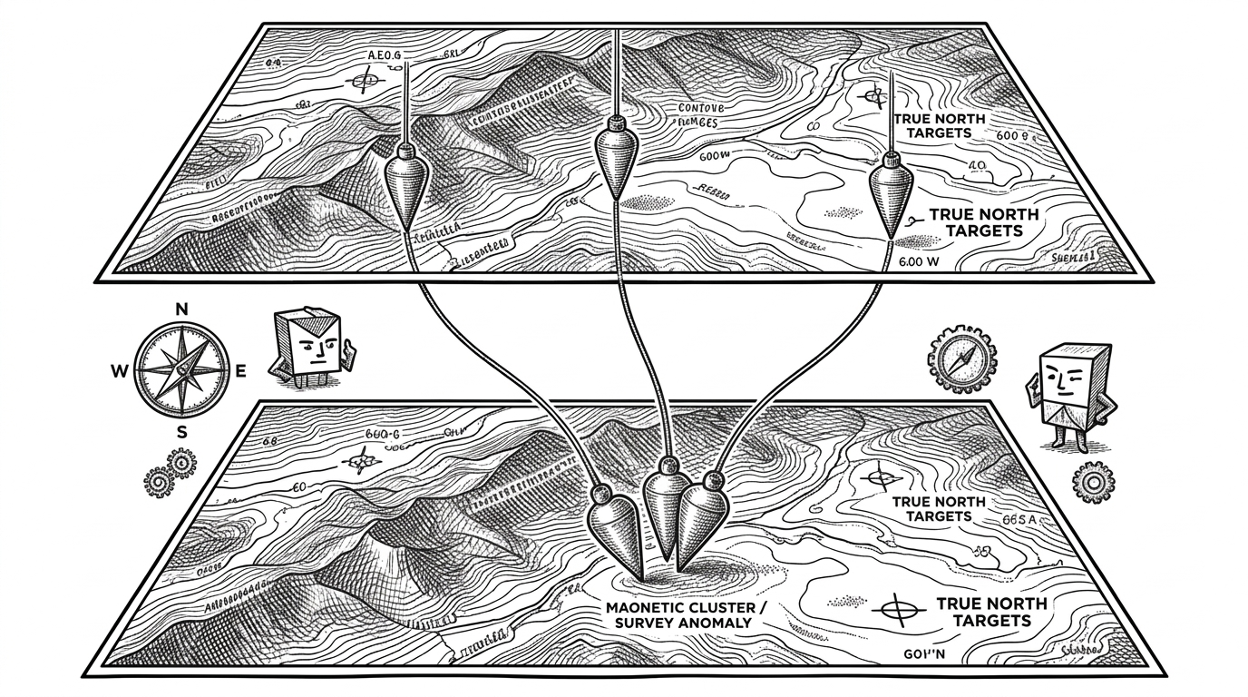
Two topographical maps stacked vertically, separated by a few inches of space. Plumb bobs drop from specific coordinates on the top map, but unseen magnetic forces bend the strings so they land clustered together on the bottom map, missing their true targets. This illustrates spatial autocorrelation. — Spatial autocorrelation warps statistical independence. Nearby geographic areas pull on each other, requiring strict clustered standard errors to prevent false confidence.

The repository goes further with 15_spatial_autocorrelation.py. It calculates Moran's I not just on the raw disease prevalence, but on the regression residuals. If the errors are clustered geographically, it signals that the model is leaking spatial data. This is defensive programming applied to pure mathematics.

A grid of squares representing census tracts

The End of the "Messy Notebook"

The true value of places-hrsn-analysis is not just in its econometric rigor. It is in how it packages that rigor for reproducibility. It replaces the fragile, exploratory nature of academic data science with the structural guarantees of software engineering.

Feature	Standard Academic Notebook	`places-hrsn-analysis` Pipeline
State Management	Hidden in-memory state, dependent on cell execution order.	Stateless, numbered Python scripts (01 to 44) persisting to disk.
Configuration	Variables hardcoded and scattered across multiple cells.	Centralized `params.yml` governing all downstream logic.
Data I/O	Raw `pd.read_csv` calls with silent data dropping.	Defensive I/O wrappers that automatically log dataframe shape changes.
Spatial Awareness	Basic OLS assumptions, ignoring geographic reality.	County-clustered standard errors and Moran's I residual checks.

By treating epidemiology as a data engineering discipline, the project ensures that its conclusions about health disparities are driven by real-world signals, not by the statistical echoes of synthetic data.

Sources:

Repository: yoelplutchok/places-hrsn-analysis
CDC PLACES Data overview and methodology.