nhr_lstm_mpc: When a Robot’s Memory Becomes Part of the Controller
A learned-dynamics control stack for nonholonomic robots that combines angle-safe physics, residual sequence models, and MPC or MPPI inside one research framework.
- nhr_lstm_mpc treats learned memory as part of the controller state, not as an external predictor bolted on afterward.
- Its most practical trick is angle-safe state design, because cos and sin avoid the discontinuity that breaks naive learned dynamics.
- The repo pairs residual dynamics with two different memory strategies, an LSTM and a history-window MLP, so control can choose between sequence state and simpler feature history.
- MPC and MPPI are presented as different ways to exploit the same learned model, one solver-driven and one sampling-driven.
The best way to read nhr_lstm_mpc is not as a neural-network project. It is a control project that refuses to pretend memory does not exist. The repo’s central idea is simple and sharp: if the learned dynamics need history, the controller has to inherit that history too.
The controller is not blind to memory
Most learned-control systems make the same quiet assumption: the next step depends only on the current state. That works until the robot’s behavior depends on unobserved momentum, delayed effects, or any other history-sensitive detail. This repo breaks that assumption on purpose.
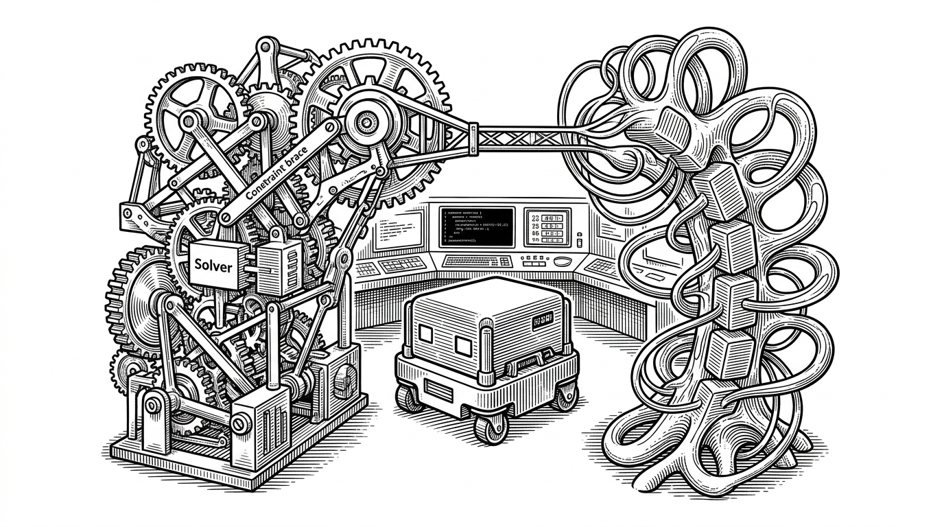
In the LSTM path, the solver does not receive a plain plant state. It receives an augmented state that includes the neural network’s hidden and cell state, so the optimization loop can carry memory forward instead of dropping it between timesteps. That is the real bridge in this project.
The implication is bigger than one architecture choice. The controller is no longer asking a black box for a prediction and hoping the internals stay stable. It is treating memory as a first-class control variable.
Why the physics layer uses cos and sin instead of angles
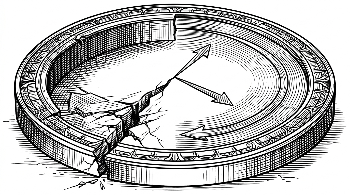
The repo’s state design is doing more work than it first appears. For heading, it uses cos θ and sin θ instead of a raw angle, which avoids the wraparound seam at 2π and keeps the learned model from seeing a fake discontinuity.
def ss_disc_sincos_nhr(x, u, dt):
    # x contains position, velocity, cos(theta), sin(theta)
    # propagate the robot without ever exposing a wrapped angle seam
    x_next = dynamics_step(x, u, dt)
    x_next[2:4] = normalize_sincos(x_next[2:4])
    return x_next
Two ways to learn motion
The repository keeps two learned-dynamics strategies side by side. One is an LSTM that carries latent state forward. The other is a history-window MLP that sees a fixed slice of past inputs and observations. Both predict residuals instead of absolute positions, which makes the model less brittle and more position-invariant.
| Model | Memory shape | What it is good at | Trade-off |
|---|---|---|---|
| LSTMDynamicsModel | Hidden state and cell state | Learning sequence effects that do not fit in a fixed window | Needs warmup and careful state management |
| HistoryMLPModel | Concatenated history window | Simple, explicit feature engineering and easier reasoning | Can miss long-range temporal effects |
| Residual prediction | Delta state output | Generalization across map position | Depends on good state normalization |
That comparison matters because the repo is not worshipping one model family. It is testing two different answers to the same control problem. If the robot’s behavior is genuinely sequential, the LSTM earns its keep. If a smaller history slice is enough, the MLP path is easier to inspect.
What warmup really fixes
Recurrent models are not ready to control on the first tick. They need context to reconstruct their internal state, which is why the warmup routine matters. Before the controller starts making decisions, the model digests recent history so its hidden state stops being random noise.
state = lstm_model.warmup(history)
action = controller.solve(state)
next_state = lstm_model.step(state, action)
That is a small piece of plumbing with big consequences. Without it, the controller would optimize against a model that has not yet remembered enough to be useful.
How the learned model enters MPC
The bridge into control happens in the wrapper layer and the Acados integration. The learned network has to be translated into a form the solver can consume, differentiate through, and stabilize. That is where tools like l4casadi matter, because they turn a PyTorch model into something a symbolic optimizer can actually use.
This is also where the repo gets practical. Learned Jacobians can be ugly, so the code adds regularization to keep the optimizer from getting lost in its own math. The result is not just a neural controller. It is a controller that behaves like it expects numerical friction.
Sampling against solving
The repo offers two control philosophies on top of the same learned dynamics. MPC searches for a locally optimal solution under constraints. MPPI samples many candidate trajectories and ranks them by cost. Both are useful, but they fail in different ways.
| Controller | How it thinks | Strength | Weakness |
|---|---|---|---|
| MPC | Optimizes a constrained horizon | Disciplined and structured | Sensitive to model smoothness and solver conditioning |
| MPPI | Samples and reweights trajectories | More forgiving with messy learned models | Can be compute-heavy |
| Shared learned model | Same dynamics interface | One model, two controller styles | Requires careful wrapper design |
That side-by-side setup is the article’s real comparison story. The repo is not choosing a winner. It is showing that the same memory-aware dynamics can support both a solver-driven controller and a sampling-driven one.
Why this repo feels like a research template
The codebase reads like a reusable stack, not a one-off demo. Data generation, model training, warmup, wrappers, MPC, MPPI, and simulation are separated into different files, which makes the research logic legible. That matters because learned control only becomes useful when the pipeline is inspectable.
The deeper value here is architectural discipline. The repo shows how to combine system identification, residual dynamics, state encoding, and solver-based control without collapsing everything into one opaque script.