2D-Surface-Mapping-SLAM and the Kalman Filter That Fuses the Wrong Signal
The README promises a Bluetooth SLAM robot with an IMU and a motor driver. The code is five kilobytes that draw a very convincing map of nothing.
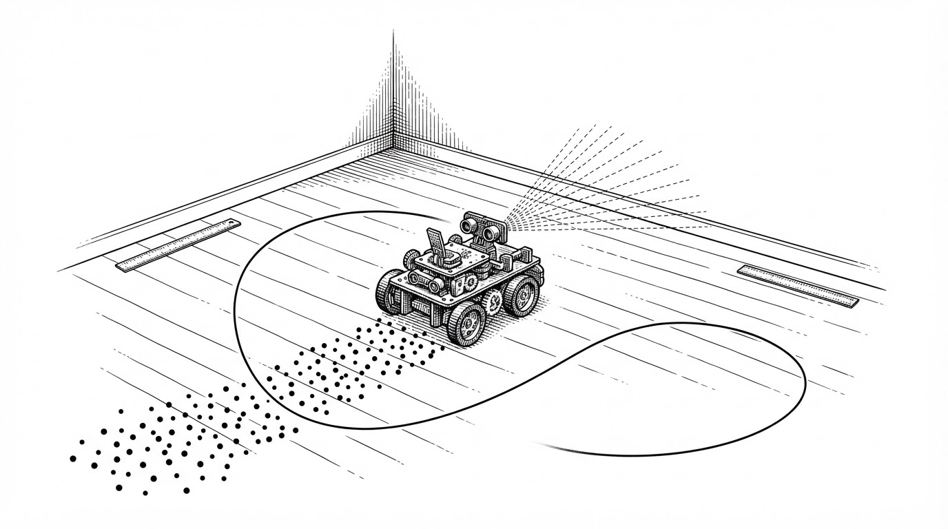
- The README describes a Bluetooth SLAM robot with an IMU and a motor driver, but the repository contains a serial reader, two filters, a geometry function, a plotter, and a logger.
- The Kalman filter declares it measures position with H = [1, 0] and is handed acceleration, so it smooths the wrong quantity and returns a plausible number with the wrong units.
- The committed sensor_data.csv matches the random distributions in test_main.py, which suggests the sample map was generated by the simulator rather than recorded from hardware.
- A pipeline that runs, plots, and logs is not the same as a correct one, because the failure mode of a mis-specified model is a nice-looking graph, not a crash.
Five kilobytes, four claims
The repository is called 2D-Surface-Mapping-SLAM. Its README describes a Bluetooth-controlled robot carrying an MPU-9250 IMU, an HC-SR04 ultrasonic sensor, and a motor driver. That is a reasonable spec for a low-cost indoor mapping platform. It is also, as far as the supplied file set goes, a spec and nothing more.
There is no firmware, no Bluetooth code, no motor control, and no IMU driver. The file named imu.py never touches an IMU. It reads a line of text off a serial port and splits it on commas. The file named test_main.py contains no tests. This needs saying fairly: the firmware may live in another repository, and the README may be a statement of intent rather than a description. What is certain is that the code here cannot drive a robot.
What the repository does contain is a pipeline. A serial reader parses four floats per line. Two Kalman filters produce a cart position. A geometry function turns range and bearing into a Cartesian point. A plotter draws the points and a smoothed curve over them. A logger appends each row to a CSV. Five modules, clean boundaries, roughly five kilobytes of Python.
| Claimed in README | Present in repo? | Where it lives |
|---|---|---|
| Bluetooth control | No | Not present in the supplied file set |
| MPU-9250 IMU driver | No | imu.py parses serial text only |
| Motor control | No | Absent |
| ESP32 firmware | No | Absent |
| Localization | Partly | kalman.py, but it fuses the wrong signal |
| Mapping algorithm | Partly | ultrasonic.py plus plotter.py |
| Tests | No | test_main.py is a simulator with no assertions |
The filter that fuses the wrong signal
Here is the centerpiece. The Kalman filter is configured as a two-state constant-velocity model, estimating position and velocity. The state transition matrix F advances position by velocity over a 0.1 second step. The measurement matrix H = [1, 0] declares that the sensor observes position, which is state index zero.
def init_kalman_filter():
    kf = KalmanFilter(dim_x=2, dim_z=1)
    kf.F = np.array([[1, 0.1], [0, 1]])   # constant-velocity model, dt = 0.1
    kf.H = np.array([[1, 0]])             # measures position (state[0])
    kf.P *= 1000
    kf.R = 0.1
    kf.Q = np.array([[0.1, 0], [0, 0.1]])
    kf.x = np.array([[0], [0]])
    return kf

def update_position(kf_x, kf_y, ax, ay):
    kf_x.predict(); kf_y.predict()
    kf_x.update(ax); kf_y.update(ay)
    x_cart, _ = kf_x.x
    y_cart, _ = kf_y.x
    return float(x_cart), float(y_cart)
Read the last two lines of update_position. The value passed to update() is ax, an acceleration. The model has just been told that this quantity is a position. So the filter fuses acceleration as if it were position, and hands back a smoothed, lagged version of acceleration labeled x_cart.
A correct model would treat acceleration as a control input, route it through the B matrix with a dt²/2 term, integrate it into velocity, and integrate velocity into position. The code does none of that. It is not a filter that is slightly off. It is a filter estimating a quantity the rest of the pipeline then mistakes for a location.
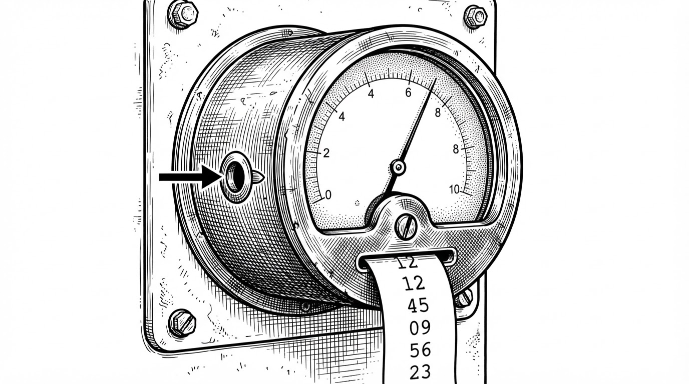
The reason this survives is that it does not throw. A mis-specified Kalman filter does not crash, does not warn, and does not produce obviously wrong numbers. It produces smooth numbers. In the committed sample data, X_Cart reads 0.467 exactly where Ax reads 0.467. The output tracks the input almost one to one, which is the fingerprint of a smoother, not an estimator.
A smoothed curve through a point cloud
Two smaller errors share a shape with the first: a correct tool applied to the wrong kind of input. Both are quiet. Neither throws.
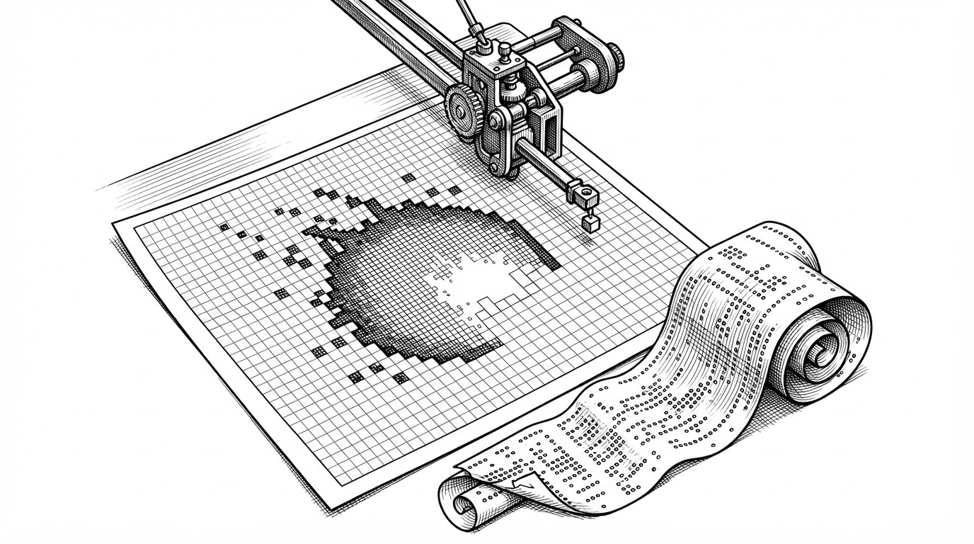
The plotter draws a red line labeled Smoothed Surface using scipy.signal.savgol_filter. Savitzky-Golay smoothing assumes an ordered signal, where neighboring samples are neighbors in the domain being smoothed. The points arrive in time order, not spatial order. So the red curve is a smoothed line drawn through scattered points in the order they happened to be measured. It is not a surface, and the label is misleading.
Then there is the missing transform. The one genuinely SLAM-shaped function in the repository is the range-and-bearing conversion, and it is correct arithmetic.
def polar_to_cartesian(x_cart, y_cart, distance, angle):
    x = distance * np.cos(np.radians(angle)) + x_cart
    y = distance * np.sin(np.radians(angle)) + y_cart
    return x, y
This converts a range and bearing into a world point, offset by the cart position. It is right for a sensor at the cart with a world-aligned bearing. What it never does is rotate the bearing from the robot frame into the world frame. There is no heading channel anywhere in the pipeline, and the protocol carries no yaw. The moment the robot turns, every point is wrong, because the bearing is still measured against a fixed axis the robot has left behind. A robot that only ever drives straight could use this. A mapping robot cannot.
The data file that wrote itself
The repository ships a file called sensor_data.csv. It has 35 rows and four fields. It looks like a log. Here is what it looks like on closer inspection: acceleration values fall in the range minus one to one, distances fall between 5 and 50, angles fall between 0 and 360, and the timestamps cluster at one-second resolution with several rows per second.
Now read the simulator. test_main.py draws random.uniform(-1, 1) for the accelerations, random.uniform(5, 50) for distance, and random.uniform(0, 360) for angle, then sleeps 0.1 seconds per iteration. Those are the same ranges. That is the same cadence. The committed data matches the simulator's output distribution, which is a strong indication that the sample map was generated by the harness rather than recorded off a robot. This is an inference from the numbers, not a proven fact. The PDF report and the commit history would settle it.
The lesson generalizes past this repo. Before you cite a dataset, look at its provenance. Real sensor data carries quantization, drift, dropouts, and a units column. Synthetic data carries round numbers and suspiciously clean ranges. When a CSV's values sit inside the exact bounds of a random call, you are reading a program, not a robot.
What real 2D SLAM actually does
It is worth naming the systems this project is measured against, because the gap is instructive. Each of these solves a specific problem, and none of those problems is solved in the repository. That is not a scandal. The repository never claims to be any of them.
| Project | Core approach | Odometry required | Loop closure | Problem it solves |
|---|---|---|---|---|
| GMapping | Rao-Blackwellized particle filter | Yes | No | 2D occupancy grids from laser scans |
| Hector SLAM | Multi-resolution scan matching | No | No | Mapping when odometry is unreliable |
| Cartographer | Graph SLAM with submaps | Yes | Yes | Large-scale 2D and 3D maps |
| SLAM Toolbox | Graph SLAM on Open Karto | Yes | Yes | Production ROS mapping and localization |
| This repo | Serial plotter | No | No | None of the above |
GMapping builds an occupancy grid with a particle filter. Hector SLAM matches scans against a multi-resolution map and can run without wheel odometry at all. Cartographer assembles submaps and closes loops to keep large maps consistent. SLAM Toolbox takes the Open Karto lineage into ROS and adds serialization, localization, and map merging. Every one of them is answering the question this project never asks: how do you keep a map consistent when the pose estimate drifts.
This package contains the ability to do most everything any other available SLAM library, both free and paid, and more.
What is worth keeping
The honest close is that this repo is a readable skeleton, and skeletons matter. The module boundaries are clean: acquisition, filtering, geometry, plotting, and logging are separated, and you can follow the data flow in one sitting. The range-and-bearing function is a tidy teaching example in isolation. The kf.P *= 1000 line is a conventional and correct way to say the initial state is unknown. The serial parser fails cleanly on the wrong field count.
The fix list is short, which is the good news. Each item is small, and each one is the kind of mistake that only looks obvious once you know to look.
- Route acceleration through the B matrix as a control input, then integrate once for velocity and again for position, instead of feeding it to update() as a measurement.
- Add a heading channel to the protocol and rotate the bearing from the robot frame into the world frame before converting to Cartesian.
- Stop truncating sensor_data.csv at import time in logger.py, and open the file in append mode so a prior run survives the next one.
- Replace savgol_filter on unordered points with smoothing that respects spatial neighbors, or drop the Smoothed Surface line until you have one.
The portable lesson is not about this robot. It is about how a pipeline that runs is not the same as a pipeline that is correct, and how the failure mode of a mis-specified model is a smooth, confident, believable graph. The next time a plot looks good, check the units before you trust the map.